Tutorial: GW for Graphene, Start to Finish
This tutorial follows one complete calculation — the extended-Hubbard model of
graphene solved in the GW approximation — from problem formulation through
input construction, execution, HDF5 output inspection, post-processing, and
physical interpretation. All files are in
examples/graphene/
of the repository, and the whole workflow is two commands:
cd examples/graphene
qassemble            # ~20 s serial
python analyze.py    # band structure, DOS, Matsubara Green's function
1. The model
Graphene is described by a two-site honeycomb lattice with one orbital per carbon sublattice. The Hamiltonian is the extended Hubbard model
with nearest-neighbour hopping \(t = 1.0\) eV, on-site interaction \(U = 2.0\) eV, and nearest-neighbour interaction \(V = 0.2\) eV, at half filling — the parameters of the graphene results section of the QAssemble manuscript. See the Hamiltonian and GW approximation theory pages for the formalism.
2. The input file
examples/graphene/qassemble.in is a single declarative dictionary with
three sections. The parser accepts only literal data — no code is executed
(see the quick start for the format
rules).
Crystal defines the geometry and electron count:
"Crystal": {
    "RVec": [[1, 0, 0], [0.5, 0.866, 0], [0, 0, 1]],   # hexagonal lattice vectors
    "Basis": [[[0.33333, 0.33333, 0], 1],              # sublattice A: position, 1 orbital
              [[0.66667, 0.66667, 0], 1]],             # sublattice B
    "CorF": "F",          # basis positions are fractional
    "NSpin": 1,           # spin-unpolarized
    "NElec": 2,           # electrons per unit cell -> half filling
    "KGrid": [25, 25, 1], # Monkhorst-Pack mesh
},
Hamiltonian holds the one- and two-body terms. Keys are tuples
(site, orbital); each hopping/interaction amplitude maps to the list of
lattice translations it connects:
"OneBody": {
    "Hopping": {
        ((0, 0), (1, 0)): {                       # sublattice A orbital 0 -> B orbital 0
            1.0: [[0, 0, 0], [-1, 0, 0], [0, -1, 0]],  # t (eV): three NN vectors
        },
    },
    "Onsite": {0: {(0, 0): 0.0, (1, 0): 0.0}},
},
"TwoBody": {
    "Local":    {...},                            # U = 2.0 eV per site (Slater-Kanamori)
    "NonLocal": {((0, 0), (1, 0)): {0.20: [...]}} # V = 0.2 eV on the same NN vectors
},
Control selects the method and numerical parameters:
"Control": {
    "Method": "gw",          # 'tb', 'hf', or 'gw'
    "Prefix": "graphene",    # output file: graphene.h5
    "NSCF": 2000,            # max self-consistency iterations
    "Mix": 0.1,              # linear mixing weight
    "T": 2000,               # temperature (K); sets beta for the DLR
    "MatsubaraCutOff": 100,  # DLR energy cutoff (eV)
    "ConstantW": 1.0,
},
3. Running
The log prints one block per iteration. Watch for the convergence criteria and the chemical potential:
iteration : 34
fcriteria : 7.57e-07        # max change of the fermionic quantities
bcriteria : 1.95e-06        # max change of the screened interaction W
chemicalpotential : 1.5999999636787783
Self-consistency is achived with 34-th
The calculation converges in 34 iterations (~20 s serial) and closes with the total GW loop time.
4. The HDF5 output
Everything is stored in graphene.h5. The layout is
/<method>/<Class>/<dataset>:
graphene.h5
├── input/                  # verbatim copy of the parsed input sections
└── gw/
    ├── H0/h0k              # (2, 2, 1, 625)      non-interacting H(k)
    ├── V/vk                # bare interaction
    ├── G0/g0kf             # (2, 2, 1, 625, 40)  bare G on the DLR nodes
    ├── G/gkf, mu, gkf.{n}  # interacting G, chemical potential
    ├── SigH/sigmah{.n}     # Hartree self-energy
    ├── SigF/sigmaf{.n}     # Fock self-energy
    ├── SigGWC/sigmagwckf{.n}  # dynamic GW self-energy
    ├── P/pkf{.n}           # polarization
    └── W/wkf{.n}           # screened interaction
Two conventions to know:
- Unsuffixed datasets are the converged result; a
.nsuffix (gkf.3,sigmah.2, …) is the per-iteration history. - Array axes follow
(norb, norb, nspin, nk[, nfreq]). The last axis of dynamic quantities runs over the ~40 DLR Matsubara nodes, not a uniform frequency grid — the DLR page explains why so few points suffice.
Any HDF5 tool works for a first look (h5ls -r graphene.h5, or h5py as
below).
5. Post-processing
examples/graphene/analyze.py contains the complete analysis; run it with
python analyze.py. The pieces are shown here.
Loading results and rebuilding the geometry
The path classes FPathStc/FPathDyn reconstruct the Crystal (and the
DLR basis) directly from the /input section of the HDF5 file, and
Crystal.Kpath sets up the high-symmetry path
\(\Gamma \to K \to M \to \Gamma\):
import h5py
from QAssemble import FPathDyn, FPathStc

fpathstc = FPathStc(hdf5file="graphene.h5")
fpathstc.crystal.Kpath(kpath=[[0, 0, 0], [2/3, 1/3, 0], [1/2, 1/2, 0], [0, 0, 0]], nk=121)
fpathdyn = FPathDyn(hdf5file="graphene.h5")   # also rebuilds the DLR

with h5py.File("graphene.h5", "r") as h5:
    h0k = h5["/gw/H0/h0k"][()]
    mu = h5["/gw/G/mu"][()]
    # ... sigmah, sigmaf, sigmagwckf, gkf
Band structure: interpolating onto the path
A static k-space matrix is moved onto the path by Fourier transforming to real space and back onto the path points, then diagonalizing:
mat_r = fpathstc.flatstc.K2R(h0k)
mat_path = fpathstc.R2K(matr=mat_r, kpoint=fpathstc.crystal.kpath)
tb_band = fpathstc.flatstc.Diagonalize(mat_path)
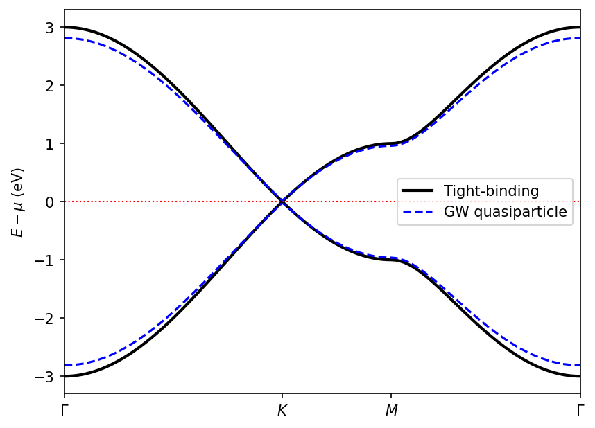
Quasiparticle bands from the GW self-energy
The dynamic self-energy \(\Sigma^{GW}(k, i\omega_0)\) at the first Matsubara frequency is split into its Hermitian part (a static level shift) and its anti-Hermitian part, which gives the quasiparticle weight
analyze.py::qp_hamiltonian implements this (with a check that the Z
eigenvalues lie in \([0, 1]\)); the result is diagonalized on the path exactly
like the tight-binding matrix.
Density of states
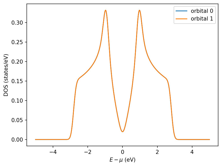
FPathStc.Dos takes the real-space matrix, samples a dense k mesh, and
returns the Gaussian-broadened, orbital-resolved DOS:
The Matsubara Green's function
Dynamic quantities live on the DLR nodes. To plot them, fit the DLR expansion and evaluate on a uniform Matsubara grid:
omega_uniform = fpathdyn.dlr.MatsubaraFermionUniform()
g_uniform = fpathdyn.dlr.MatsubaraDLR2Uniform(gkf[0, 0, 0, ik_gamma, :])[:, 0, 0]
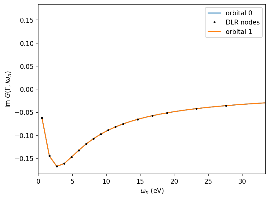
The ~20 positive-frequency DLR nodes (dots) reproduce the full smooth frequency dependence (line) — this compression is what makes the GW loop cheap.
6. What the results mean
- The GW bands stay close to the tight-binding bands. At \(U/t = 2\) graphene remains weakly correlated at this temperature: the printed Z-factor eigenvalues are \(\approx 0.94\), i.e. only mild mass renormalization (visible as a slight narrowing of the bands), and the Dirac crossing at \(K\) stays pinned to the Fermi level (\(\mu = 1.6\) eV absorbs the Hartree--Fock shift; the converged value is pinned by the reproduction test run in CI).
- The DOS shows the Dirac cone and van Hove singularities. The linear \(|E|\) onset around \(E = \mu\) reflects the Dirac dispersion; the peaks at \(\pm t = \pm 1.0\) eV are the van Hove singularities at the \(M\) point. Both sublattice orbitals are identical by symmetry.
- \(\operatorname{Im} G(\Gamma, i\omega_n)\) decays as \(-1/\omega_n\) at large frequency (the exact sum-rule tail) and remains small at low frequency because \(\Gamma\) is far from the Fermi surface.
Real-frequency spectral functions
Computing \(A(k, \omega)\) on the real axis requires analytic continuation of the Matsubara data, which is beyond the scope of this tutorial and of the QAssemble core; support for an external continuation workflow is planned.
7. Where to go next
- Change
Methodtotborhfinqassemble.in(and thePrefix) to compare the levels of theory — the sameanalyze.pyband machinery works on/tb/H0/h0kand/hf/H/hk. - The end-to-end pipeline of this tutorial runs in CI: the fast variant in
tests/test_integration_run.pyand the full manuscript reproduction intests/test_reproduce_manuscript.py.